Overview
We forecast conflict fatalities at 1–6 month horizons using shape‑based analog forecasting: we identify historical trajectories that resemble the present (via dynamic time warping, DTW), propagate them forward to retrieve their realized futures, and average those futures to produce point forecasts with calibrated uncertainty. The same design extends to subnational PRIO‑GRID (0.5°) for diffusion and hotspots.
Data
- Outcome: Monthly conflict fatalities from UCDP GED ("best" estimates), aggregated to country‑month and PRIO‑GRID cell‑month, 1989–present.
- Processing: Cleaning, harmonization, and aggregation to consistent spatial units and monthly periods.
- Refresh: Forecasts update when source data refresh.
- Optional covariates: Population & access, climate anomalies, night‑lights, governance, economy, and spatial lags.
Methods
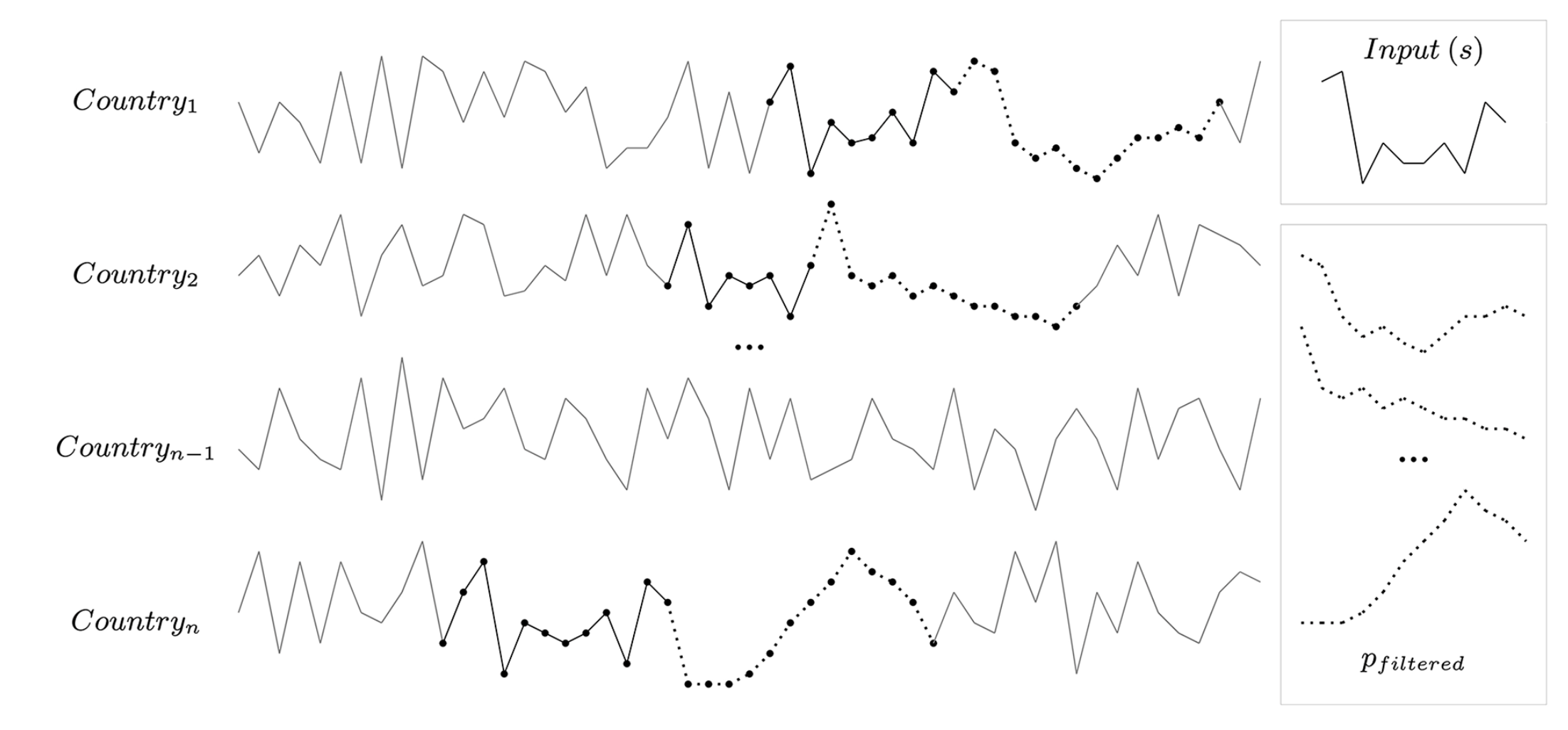
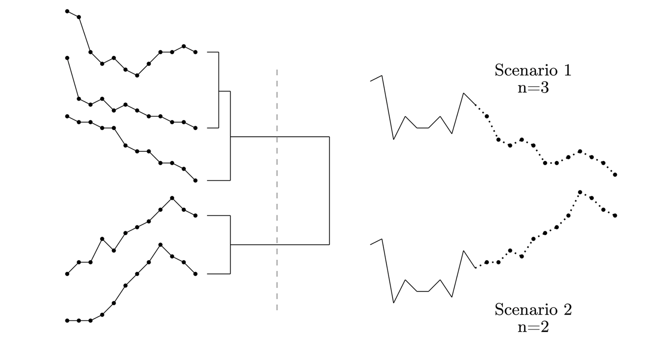
Given a recent window of outcomes for a country or grid cell, we measure similarity to all historical windows using dynamic time warping (DTW), which aligns sequences that evolve at different speeds. We then select the K nearest analog windows and follow each one forward in time to obtain its realized outcomes at horizons h = 1…6 months. These horizon‑specific sets of analog outcomes constitute an empirical predictive distribution from which we derive point forecasts (centroids) and uncertainty summaries (medians, 50/80/95% intervals, exceedance risks).
When covariates are available (e.g., demography, access, climate, economy), they can be incorporated into the similarity search, but purely autoregressive matching performs competitively at short horizons. Calibration is monitored via coverage, PIT histograms, and CRPS, with optional similarity weighting as a deployment refinement.
- Window the recent trajectory (normalize as appropriate).
- Measure similarity with DTW; select the K nearest historical windows.
- Propagate each matched window forward to collect outcomes for horizons h = 1..6 months.
- Aggregate across matched futures (centroid) for the point forecast.
- Use the set of matched futures as an empirical distribution for uncertainty.
Data Collection
UCDP conflict events, 1989–present, aggregated to countries & 0.5° grid cells
Feature Engineering
Extract covariates: demographics, climate, economy, governance, spatial lags
Pattern Matching
DTW finds similar historical trajectories
Forecast Generation
Cluster futures and compute centroid for 1–6 month predictions
Validation
Out-of-sample testing and real-world performance monitoring
Alignment Intuition
DTW aligns sequences unfolding at different speeds to expose common structure.
Why Shape‑Based Analog Forecasting
We treat each evolving trajectory (country or grid cell) as a shape in time and search the historical record for similar shapes. Those closest historical analogs provide plausible futures that we aggregate into a forecast with uncertainty.
Concretely, given a recent window of outcomes, we use dynamic time warping (DTW) to align sequences at different speeds and identify nearest analogs in the archive. We then follow each analog forward to obtain a set of candidate futures. Averaging these futures yields a strong, transparent short‑horizon forecast; the spread gives intervals and exceedances. See EPJ Data Science and the JPR paper on variability.
When covariates are available (e.g., population, access, economics, climate), we can enrich the similarity search. But a key result across our studies is that purely autoregressive shape‑matching — using only past fatalities or event intensity — performs on par with richer feature sets for short‑horizon forecasts. See also our unrest and migration applications using the same pattern‑based strategy.
Uncertainty
For each horizon h, the matched futures define an empirical predictive mixture. With equal weights 1/K, we report medians, 50/80/95% intervals, and exceedance probabilities. Calibration is monitored via coverage, PIT, and CRPS.
Subnational Modeling
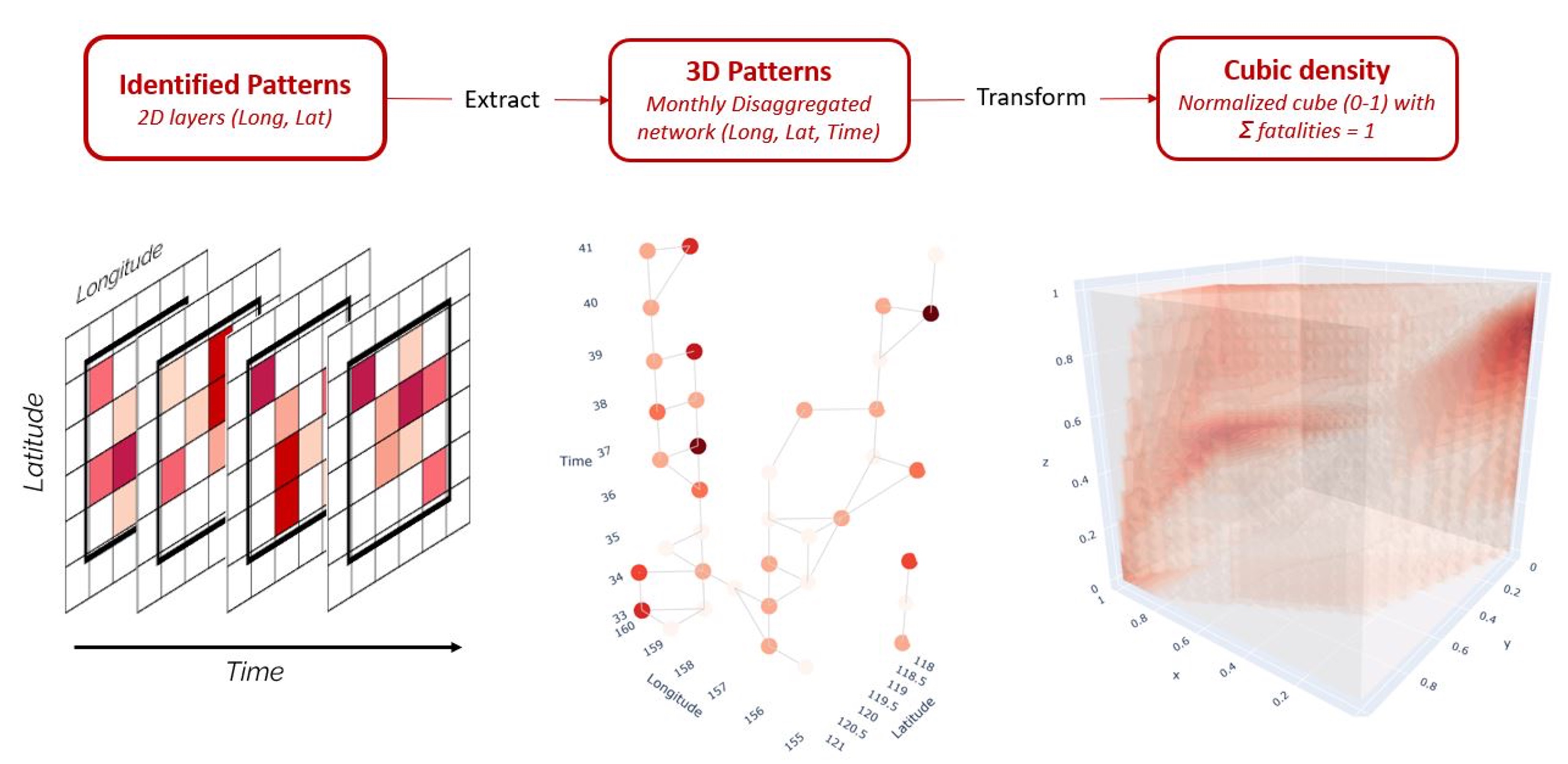
We model how risk appears, persists, and spreads across adjacent PRIO‑GRID (0.5°) cells. The method combines local history with neighborhood exposure to recover waves of escalation and hotspot formation that national aggregates can hide.
How the diffusion mechanism is captured
- Units: PRIO‑GRID 0.5° cell‑months with local lag history.
- Neighborhood exposure: Distance‑decayed activity within 1–3 cells, optionally weighted by roads/travel time.
- Front dynamics: Distance to most recent events; advancing vs receding fronts.
- Grid‑level analogs: Match cell‑windows on local+neighbor patterns; use their subsequent outcomes to form a predictive mixture.
Validation
- Generalization: Patterns recur across geographies and epochs; models retain accuracy out‑of‑country/region/period.
- Short‑horizon strength: Purely autoregressive shape‑matching performs on par with covariate‑rich variants.
- Explaining variation: Captures timing/magnitude of surges and lulls that linear baselines smooth.
How to Cite
Suggested citation: Schincariol, Frank & Chadefaux (2025). Accounting for variability in conflict dynamics. Journal of Peace Research. https://doi.org/10.1177/00223433251330790
@article{schincariol2025jpr,
  author = {Schincariol and Frank and Chadefaux},
  title = {Accounting for variability in conflict dynamics},
  journal = {Journal of Peace Research},
  year = {2025},
  doi = {10.1177/00223433251330790},
  url = {https://journals.sagepub.com/doi/10.1177/00223433251330790}
}
Questions & Answers
Are the patterns specific to a country, region, or epoch?
No. We explicitly test out‑of‑country, out‑of‑region, and out‑of‑period generalization and find that core shapes recur across contexts. Because alignment handles speed differences, the model recognizes the same dynamics when they unfold faster or slower, or in different decades. See our Predictability working paper.
Do you make subnational predictions?
Yes. We produce PRIO‑GRID (0.5°) forecasts alongside country‑level outputs. The grid approach captures local persistence and spillovers, and is visualized via 3D space–time shapes and diffusion animations. See the 3D shapes working paper in our Working Papers.
How does the autoregressive baseline compare?
For short horizons, a purely autoregressive, shape‑matching approach performs on par with covariate‑augmented versions. This makes the baseline attractive when exogenous data are delayed or noisy, and provides a strong, transparent reference for practitioners. See EPJ Data Science and the Journal of Peace Research paper on accounting for variability.
What do we explain particularly well?
Variation over time — especially the onset, escalation, and decay of episodes. By using analog futures from the closest matches, the model captures bursts and plateaus that standard linear baselines often smooth out. See our Journal of Peace Research paper on accounting for variability.
Is this causal or predictive?
Predictive. We focus on anticipating outcomes given current trajectories and historical regularities. That said, the analog set provides interpretable narratives — “this looks like these past episodes” — that support diagnostic and scenario discussions.
How do you quantify uncertainty?
Following the papers, we take the K most similar historical windows (via DTW shape matching). For each forecast horizon h, we use the matched windows’ subsequent outcomes to form an empirical predictive distribution, and we take the average (centroid) of those futures as the point forecast. Equivalently, with equal weights 1/K, the mixture is ph(y) = (1/K) · ∑k=1..K δ(y − yk,h). From this distribution we report prediction intervals (e.g., 50/80/95%) and exceedance probabilities.
We evaluate forecasts out‑of‑sample against baseline models and monitor interval coverage. In deployment, we may optionally apply similarity weighting and distributional diagnostics (e.g., PIT/CRPS) for ongoing calibration monitoring.
What horizons do you support?
Commonly 1–6 months, but the same design extends to weekly or quarterly horizons. We choose horizons based on stakeholder needs and data refresh cycles.
Does this work beyond conflict fatalities?
Yes. We use similar shape‑based methods for protest intensity and migration flows. The approach is generic to time‑series with recurring motifs and regime shifts.
Limitations
- Novelty risk when dynamics lack historical analogs.
- Data latency/quality effects propagate into forecasts.
- Predictive, not causal; analog narratives support interpretation but not attribution.
References
Appendix
For additional questions, see the FAQ.